
Geotechnical engineering libraryContact
 benesch
Primary Reference: USACE EM 1110-1-1804, Geotechnical Investigations (2001), Sections 4-5 through 4-12; ASTM D5778, D2573, D4719, D6635, D7128; AREMA Manual for Railway Engineering (MRE) Chapter 1.
Apps on dirtbert.com that support this chapter. Each one runs in a web browser on a desktop or a phone, with nothing to install. How to use the apps (I.3). Tools marked TOOLS open in the Geotechnical Analysis Suite (Benesch sign-in); the orange card below lists each one by section.
NANCY pages ask you to accept the Use and Disclaimers once in each browser.
Calculators and workbook tools from the Benesch Geotechnical Analysis Suite that support this chapter: 2 interactive calculators and 3 workbook guides. Each one is also placed inside the section it supports, in an orange tools strip.
| SP | Dynamic Cone PenetrometerUsed in 7.2 Cone Penetration Test (CPT and CPTu) | Calculator ▸ | Guide |
| FF | Dynamic Cone Field LogUsed in 7.2 Cone Penetration Test (CPT and CPTu) | Calculator ▸ | Guide |
| SP | CPT–SPT CorrelationUsed in 7.2 Cone Penetration Test (CPT and CPTu) | guide only | Guide |
| SP | Vane ShearUsed in 7.3 Vane Shear Test (VST) | guide only | Guide |
| SS | Seismic Site Class DeterminationUsed in 7.6 Multichannel Analysis of Surface Waves (MASW) | guide only | Guide |
Tools open on dirtbert.com and need the Benesch sign-in. Drafts pending Benesch final review, not for use in design.
General topic illustrations from Benesch's shared geotechnical graphics library, related to this chapter's subject matter — not the numbered figures called out in the text above. Click any image to view it full size.
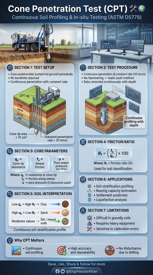
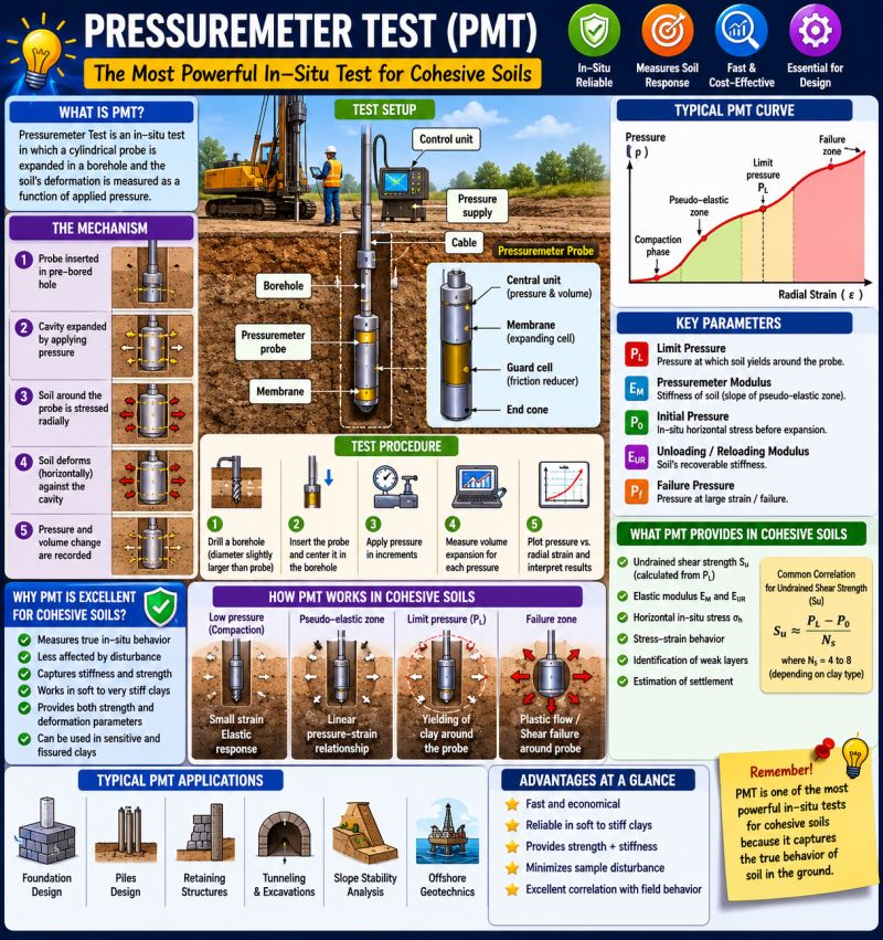

In situ testing provides continuous or near-continuous soil and rock characterization without the inherent sample disturbance associated with laboratory testing. For railroad geotechnical investigations conducted on behalf of CSXT, NSR, UPRR, BNSF, CPKC, Amtrak, CN, G&W subsidiaries, and in conformance with AREMA MRE Chapter 1, we routinely deploy six primary in situ methods: the Cone Penetration Test (CPT/CPTu), the Vane Shear Test (VST), the Pressuremeter Test (PMT), the Flat Dilatometer Test (DMT), Multichannel Analysis of Surface Waves (MASW), and seismic refraction. Each method addresses a specific subsurface condition or design need. This chapter presents the theoretical basis of each method with equations expressed in English units (psf, pcf, psi, ft, ksf), step-by-step worked calculation examples set in railroad project contexts, client-specific application guidance, a method comparison table, a field operations checklist, and five practice questions with complete answers. Cross-references to Chapter 6 (SPT corrections), Chapter 8 (soil classification), Chapter 11 (bearing capacity), Chapter 12 (settlement), Chapter 13 (slope stability), and Chapter 14 (seismic/liquefaction) are provided throughout.
Values from these correlations are estimates, not test results. State the equation ID and source when one is used, confirm the soil or rock is within its range, and calibrate against site testing before design.
The correlations below are used or referenced in this chapter. Each is a statistical fit to a particular data set, so a value from one is an estimate: it applies only within the materials and ranges stated, carries the scatter of the original data, and must be confirmed by site-specific testing or calibration before it is relied on for design.
When an equation is used, note it with the result: give the equation ID and source, state that the soil or rock is within its range of applicability, mark the value as correlated (not tested), and record the limitation that governs. The Empirical Equations & Correlations reference has every entry with its full references.
Variables. u2 = pore pressure behind cone tip; an = net area ratio (typically 0.70–0.85, from calibration)
Use. All piezocone (CPTu) soundings; essential in soft clays and silts.
Limitations. Correction negligible in clean sands; critical in soft fine-grained soils. Requires u2 filter position.
Source. Lunne et al. 1997 · In this chapter: 7.9, 7.12, 7.13, 7.14 · Full entry and references
Variables. Nkt = empirical cone factor, typically 10–20 (average ≈ 14); decreases with increasing Bq
Use. Fine-grained soils penetrated undrained (Ic > ~2.6).
Limitations. Nkt depends on reference test (vane, CIUC, DSS) and plasticity; calibrate locally. Use Nkt toward upper end for conservative Su.
Source. Lunne et al. 1997 · In this chapter: 7.9, 7.12, 7.14 · Full entry and references
Variables. Ic from IS-13
Use. Young, uncemented Holocene–Pleistocene soils.
Limitations. Underpredicts Vs in aged or cemented soils. Measure Vs directly for seismic site class.
Source. Robertson 2009 · In this chapter: 7.1, 7.8 · Full entry and references
Variables. p0, p1 = corrected A and B pressures; u0 = hydrostatic pore pressure
Use. All soils penetrable by the blade; ID < 0.6 clay, 0.6–1.8 silt, >1.8 sand.
Limitations. ED is not a design modulus; convert with MDMT = RM · ED (Marchetti 1980).
Source. Marchetti 1980 · In this chapter: Executive Summary, 7.5, 7.8, 7.12, 7.13, 7.14 · Full entry and references
Variables. KD from IS-23
Use. Uncemented, unaged clays with ID < 1.2.
Limitations. Not valid in sands, cemented, or heavily aged deposits; check against lab or vane data.
Source. Marchetti 1980 · In this chapter: 7.8 · Full entry and references
Variables. PI = plasticity index (%)
Use. Soft clays, embankment stability on soft ground; based on back-analyzed failures. Typical PI 5–100%.
Limitations. Not applicable to fissured, varved, or organic clays without local calibration. Scatter about ±25%.
Source. Azzouz et al. 1983 (fit to Bjerrum 1972) · In this chapter: 7.12, 7.14 · Full entry and references
Variables. φ' = effective friction angle
Use. Uncemented soils on primary unloading.
Limitations. Not valid on reloading or for compacted fills, where K0 is governed by compaction stresses. Cap at passive limit.
Source. Jaky 1944; Mayne & Kulhawy 1982 · In this chapter: 7.14 · Full entry and references
Variables. σ'm = mean effective stress; k = 0 (PI=0) to 0.5 (PI ≥ 100)
Use. Uncemented clays and sands; lab resonant-column basis.
Limitations. Underestimates aged/cemented soils; field Vs (Gmax = ρVs2) is preferred.
Source. Hardin 1978 · In this chapter: 7.1, 7.8, 7.12, 7.14 · Full entry and references
Variables. fs = sleeve friction
Use. All CPT data; basis for SBT classification and most Robertson-family correlations below. Ic < 2.6 ≈ coarse-grained / drained; > 2.6 ≈ fine-grained / undrained.
Limitations. SBT is behaviour type, not grain-size classification. Cemented, aged, or sensitive soils plot misleadingly. Earlier n-exponent forms exist (Robertson & Wride 1998).
Source. Robertson 2009 · Full entry and references
Variables. Bracketed term = Qt1 (normalized tip resistance)
Use. Clean, unaged, uncemented quartz sands; based on calibration chamber data.
Limitations. Overpredicts in compressible (carbonate, micaceous) sands; underpredicts in aged/cemented sands.
Source. Kulhawy & Mayne 1990 · Full entry and references
Variables. QC = compressibility factor (0.91 low, 1.00 medium, 1.09 high compressibility); t = age in years
Use. Clean quartz sands; calibration chamber database.
Limitations. Chamber size effects in dense sands; sensitive to compressibility assumption.
Source. Kulhawy & Mayne 1990 · Full entry and references
Variables. k = empirical factor
Use. Intact, inorganic clays.
Limitations. k is higher in aged/heavily OC clays and lower in fissured clays; calibrate with oedometer tests.
Source. Kulhawy & Mayne 1990; Mayne 1995 · Full entry and references
Variables. Qt = (qt − σv0)/σ'v0
Use. Uncemented soils; settlement estimates (1-D).
Limitations. Gives a representative 1-D modulus at in-situ stress; not small-strain. Organic and sensitive soils excluded.
Source. Robertson 2009 · Full entry and references
Variables. Ic from IS-13
Use. Naturally deposited soils; first-order profiling of k with depth.
Limitations. Order-of-magnitude only (±1 log cycle). Not for man-made fills; prefer CPTu dissipation t50 or field pumping tests for design.
Source. Robertson 2010 · Full entry and references
Variables. Rf = (fs/qt) × 100%; γw = unit weight of water
Use. Uncemented soils; used to build stress profiles when samples are lacking.
Limitations. Typical accuracy about ±10%; poor in organic soils, peats, and cemented layers.
Source. Robertson & Cabal 2010 · Full entry and references
Railroad embankments, bridges, culverts, and intermodal facilities impose repetitive dynamic loads that sensitize soft or marginally competent soils in ways that static design loads alone do not capture. The Cooper E-80 live load equivalent used by all Class I clients — CSXT, NSR, UPRR, BNSF, CPKC, Amtrak, and CN — combined with dynamic load factors (DLF) of 1.2 to 1.5 (see Introduction, Table I-3) means that subgrade characterization must resolve not only static strength and stiffness but also cyclic response. In situ testing is indispensable for this because:
Reference graphics · click to zoom
Access under traffic limits most in-situ tests to the shoulder or a track window. McHenry and Rose (2012) summarize the tools that can be run from the track or crib: the dynamic cone penetrometer and the instrumented French PANDA (records blow energy and penetration to give dynamic cone resistance qd), the light weight deflectometer, the German DyStaFiT dynamic plate test, and rail-bound stiffness vehicles (Track Loading Vehicle, Portancemètre). They also note that seismic CPT is attractive for railroads because a small-strain modulus better reflects the small cyclic strains under train loads than a resilient modulus does.
Source: McHenry, M. and Rose, J. (2012). Railroad Subgrade Performance Indicators — A Review of Available Testing Methods. University of Kentucky
Profillidis reproduces a matrix of in situ test methods (from Carter and Bentley, Correlations of Soil Properties) rating each method’s applicability to soil identification, profiling and engineering parameters across soil types. He notes that before 1960 the list would have held only the standard penetration test, the mechanical cone, the vane shear test and the plate load test. Today several methods can usually supply any given parameter, so the choice can be driven by soil type, depth and cost.
Figures · click to zoom
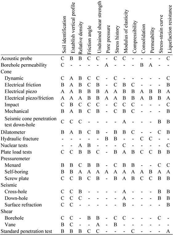
After Profillidis (2014), §9.2.3, Table 9.1; after Carter, M. and Bentley, S. (1991), Correlations of Soil Properties, Pentech Press. Full reference under Supplemental Sources.
Values from these correlations are estimates, not test results. State the equation ID and source when one is used, confirm the soil or rock is within its range, and calibrate against site testing before design.
Reference graphics
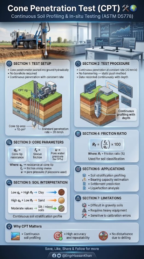
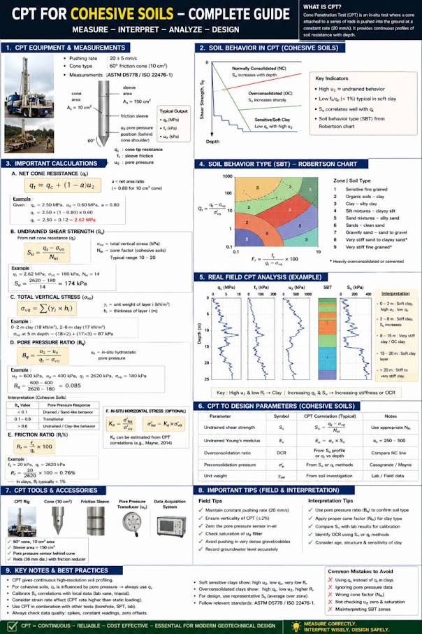
The CPT advances a 1.41-in.-diameter cone at a rate of 0.8 in./sec per ASTM D5778. The standard cone has a projected tip area of 1.55 in² and a friction sleeve area of 23.25 in². The piezocone (CPTu) adds a porous filter element — typically at the u₂ position (shoulder behind tip) — to measure pore water pressure during advancement. Amtrak ES explicitly requires CPTu (not basic CPT) for all soft-ground investigations on the NEC where settlement risk exists, citing the need for B_q pore pressure ratio data to assess consolidation state.
Measurements recorded per ASTM D5778:
For CPTu, the measured tip resistance is corrected for unequal area effects:
q_t = q_c + u₂ × (1 − a)
Where:
The friction ratio is used for soil behavior type (SBT) classification:
Reference graphics · click to zoom
R_f (%) = (f_s / q_c) × 100
Robertson (1990) SBT zones are used to classify soil type without physical samples. A simplified guide:
| SBT Zone | R_f (%) | q_c (tsf) | Typical Soil |
|---|---|---|---|
| 1 | >4 | <5 | Sensitive fine-grained |
| 2 | >3 | 5–25 | Organic / peat |
| 3 | 2–4 | 5–50 | Clay — low to medium OCR |
| 4 | 1–2 | 10–100 | Silt mixture |
| 5 | 0.5–1.5 | 50–200 | Sand mixture |
| 6 | <0.5 | >100 | Clean sand |
| 8 | <0.5 | >300 | Dense sand / gravel |
| 9 | >2 | >100 | Very stiff fine-grained |
This table is routinely incorporated into CPTu data reports delivered to CSXT, BNSF, and UPRR in their respective gINT templates.
No additional content.
Reference graphics
s_u = (q_t − σ_v) / N_kt
Where:
B_q = (u₂ − u₀) / (q_t − σ_v)
Where u₀ = hydrostatic pore pressure (tsf) = γ_w × h_w / 2,000; γ_w = 62.4 pcf, h_w = depth below water table (ft). B_q > 0.4 typically indicates soft, normally consolidated or sensitive clay — a critical flag on Amtrak NEC and CN Great Lakes alignments.
Chapter 14 presents the full liquefaction procedure; the key normalized parameter needed from CPT is:
q_c1N = (q_c / P_a) × (P_a / σ'_v)^0.5
Where:
UPRR and BNSF both accept CPT-based liquefaction screening per this method for preliminary hazard assessments on new intermodal yard sites.
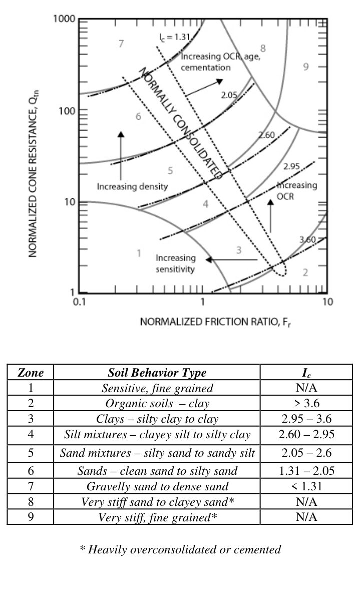
The non-normalized zones in Section 7.2.3 drift with depth because qc rises with overburden. Robertson’s normalized chart (Figure 7-S1) removes that effect and collapses the zone boundaries into one number:
Ic = [ (3.47 − log Qt)2 + (log Fr + 1.22)2 ]0.5, with Qt = (qt − σvo)/σ′vo and Fr = fs/(qt − σvo) × 100%.
| Zone | Soil behavior type | Ic | (qc/pa)/N60 |
|---|---|---|---|
| 1 | Sensitive, fine grained | N/A | 2.0 |
| 2 | Organic soils – clay | > 3.6 | 1.0 |
| 3 | Clays – silty clay to clay | 2.95–3.6 | 1.5 |
| 4 | Silt mixtures – clayey silt to silty clay | 2.60–2.95 | 2.0 |
| 5 | Sand mixtures – silty sand to sandy silt | 2.05–2.60 | 3.0 |
| 6 | Sands – clean sand to silty sand | 1.31–2.05 | 5.0 |
| 7 | Gravelly sand to dense sand | < 1.31 | 6.0 |
| 8 | Very stiff sand to clayey sand* | N/A | 5.0 |
| 9 | Very stiff fine-grained* | N/A | 1.0 |
* Heavily overconsolidated or cemented. Normalized SBT has better than 80% agreement with samples in independent studies (Robertson & Cabal, 2010). Apply the q/N ratios to qt in soft fine-grained soils.
Stopping the push and recording pore-pressure decay gives t50, the time to 50% dissipation, which yields the horizontal coefficient of consolidation (Robertson and Cabal report accuracy of about ± half an order of magnitude but excellent repeatability within a profile). Convert to vertical with cv = ch(kv/kh). Watch for dilative silts where u2 rises before it falls — run the test to true equilibrium, or measure t50 from the peak. In plastic clays dissipation can take many hours, so budget rig time accordingly on track-window-limited projects.
Robertson and Cabal recommend recording zero-load readings at the start and end of every sounding and checking wear, O-ring seals, push rods and the pore-pressure filter at the start and end of each test, with load-cell calibration at least every three months (or before and after major projects).
Source: Robertson, P. K. and Cabal, K. L. (2010). Guide to Cone Penetration Testing for Geotechnical Engineering, 4th ed. Gregg Drilling & Testing, Inc.
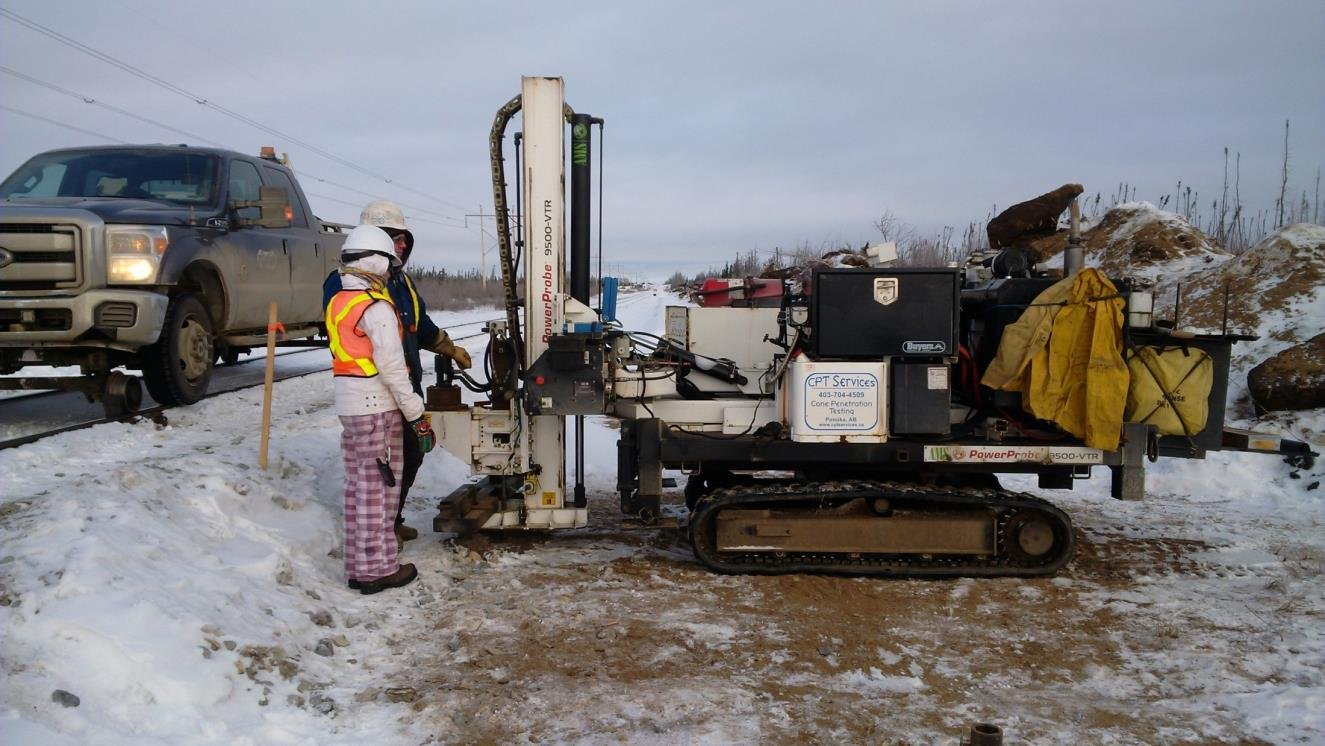
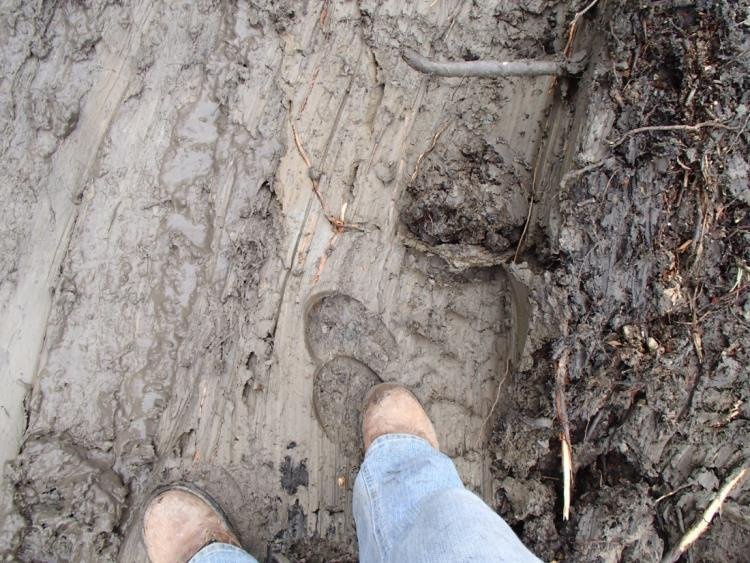
About 400 ft of track at Lac la Biche Sub Mile 173.48 was settling differentially into deep peat. Boreholes (including DH-1 and DH-3) built the stratigraphic section, and a track-mounted CPT rig filled in between them to define the depth and extent of the organic layer. The resulting design used 68 piles of 18-in. diameter, installed in two flights at 10° from vertical, to carry track load through the peat (see Chapter 11). Simple hand checks also help: at Tête Jaune Mile 40.5, clay that a thumb could penetrate several centimeters ruled out heavy equipment and rain-day work.
Figures · click to zoom

After Geotechnology for Railroaders Program, Module 6.2, Module 6.1; Module 6.2 §05; Module 6.1 §03. Full reference under Supplemental Sources.
The field vane shear test (ASTM D2573) measures peak and remolded undrained shear strength of soft to firm cohesive soils. A four-bladed vane (standard dimensions: 2.24 in. diameter × 4.49 in. height, H/D = 2) is pushed to the test depth and rotated at 6°/minute. The test is suited to soft clays with s_u < 1.0 tsf. It is inappropriate in sands, gravels, or stiff clays.
Specific applications by railroad client:
No additional content.
For H/D = 2 (standard vane):
s_u (peak) = T_peak / [π × D³ × (H/(2D) + 1/6)]
Where:
Substituting H/D = 2:
s_u (peak) = T_peak / [π × D³ × (1 + 1/6)]
= T_peak / [π × D³ × 7/6]
= 6 × T_peak / (7 × π × D³)
Converting result from lb/ft² to tsf: divide by 2,000.
Field vane s_u overestimates design undrained strength in plastic clays because the test is faster than field loading rates and the failure plane is not optimally oriented. The Bjerrum (1972) correction factor μ is applied:
s_u (design) = μ × s_u (field vane)
Where μ is a function of plasticity index (PI):
| PI (%) | μ (Bjerrum 1972) |
|---|---|
| 10 | 1.00 |
| 20 | 0.95 |
| 40 | 0.85 |
| 60 | 0.75 |
| 80 | 0.65 |
| 100+ | 0.55 |
For CSXT embankment stability analyses on Atlantic Coastal Plain soft clays (typical PI = 40–65%), μ = 0.75–0.85 is standard practice.
No additional content.
S_t = s_u (peak) / s_u (remolded)
CN Engineering Standards flag S_t > 8 as "quick clay" requiring project-level risk assessment and slope stability analysis under seismic loading per Chapter 13 and Chapter 14.
The prebored pressuremeter test (ASTM D4719) is performed in a borehole by expanding a cylindrical membrane against the borehole wall and measuring volume change versus applied pressure. The self-boring pressuremeter (SBP) minimizes disturbance but is rarely warranted on standard railroad projects. The full-displacement PMT (FDPMT) is useful in soft clays and has been used on Amtrak NEC foundation studies.
Three pressure phases define the PMT curve:
No additional content.
E_PMT = 2(1 + ν) × V_m × ΔP/ΔV
Where:
For preliminary design, E_PMT is correlated to elastic modulus of soil (E_s) for settlement analysis (Chapter 12) using E_s ≈ E_PMT / α, where α = 0.33 for OC clays and 0.67 for NC clays (Ménard 1975).
No additional content.
s_u = (p_L − p_0) / N_p
Where:
The PMT is particularly useful on NSR projects through the Appalachian ridges where borings encounter interbedded rock and soft clay, and CPT advancement is impractical.
The Marchetti flat dilatometer (ASTM D6635) is a blade with a flexible 2.36-in. diameter steel membrane pushed into the ground. Two pressure readings are taken at each depth: the "A" pressure (membrane lift-off) and the "B" pressure (membrane expansion to 0.043 in.). A third reading "C" (deflation) is optional but recommended in soft clays for pore pressure estimation.
The DMT provides three intermediate parameters:
Values from these correlations are estimates, not test results. State the equation ID and source when one is used, confirm the soil or rock is within its range, and calibrate against site testing before design.
I_D = (p_1 − p_0) / (p_0 − u₀)
K_D = (p_0 − u₀) / σ'_v
E_D = 34.7 × (p_1 − p_0)
Where p_0 and p_1 are corrected contact and expansion pressures (psf); correction equations (ASTM D6635 Annex A1) account for membrane stiffness gauge factors ΔA and ΔB.
Soil classification by I_D:
| I_D | Soil Type |
|---|---|
| < 0.6 | Clay |
| 0.6 – 1.8 | Silt |
| > 1.8 | Sand |
K_D interpretation: K_D ≈ K₀ for NC soils; K_D > 2 indicates overconsolidation. OCR ≈ (K_D / 1.5)^1.56 (Marchetti 1980) — widely applied on CSXT and BNSF soft-ground projects.
No additional content.
M_DMT = R_M × E_D
Where R_M is a correction factor (dimensionless):
M_DMT is analogous to 1/m_v used in Terzaghi consolidation theory and can substitute for oedometer data in settlement calculations (Chapter 12) when tube sampling is impractical.
Reference graphics
Reference graphics · click to zoom
MASW (ASTM D7128) measures the dispersion of Rayleigh surface waves to derive a shear-wave velocity (V_s) profile with depth. A linear array of 24 or more 4.5-Hz vertical geophones spaced 3.3–9.8 ft apart is deployed at the surface. An impact source (sledgehammer, weight drop) generates surface waves. The dispersion curve is inverted to yield V_s versus depth.
MASW offers a non-invasive site characterization option that UPRR and BNSF have increasingly required for mainline subgrade rehabilitation projects where track occupancy windows preclude drilling. CPKC has incorporated MASW into its track-structure interaction studies on prairie mainline segments. CN uses MASW extensively for permafrost boundary mapping and muskeag (peat bog) thickness profiling in Canadian operations.
No additional content.
G_max = ρ × V_s²
Where:
Example: For a sand with γ = 120 pcf and V_s = 820 ft/s:
G_max is the input stiffness for dynamic track-subgrade interaction models used by UPRR and BNSF for high-axle-load corridors (315K GRL).
The AASHTO seismic site classification is based on the time-averaged shear-wave velocity in the upper 100 ft, V_s,30:
V_s,30 = Σd_i / Σ(d_i / V_si)
Where d_i and V_si are thickness (ft) and shear-wave velocity (ft/s) of each layer in the upper 100 ft.
| Site Class | V_s,30 (ft/s) | Description |
|---|---|---|
| A | > 5,000 | Hard rock |
| B | 2,500–5,000 | Rock |
| C | 1,200–2,500 | Very dense soil / soft rock |
| D | 600–1,200 | Stiff soil |
| E | < 600 | Soft clay |
| F | — | Special study required |
All AREMA MRE Chapter 8 seismic bridge design and UPRR, BNSF, CSXT, NSR, CN, and Amtrak seismic analysis protocols reference AASHTO site class directly. MASW is the most practical tool for establishing site class when bedrock is too deep for refraction and borings are not available at every bridge location.
Reference graphics
Seismic refraction measures the first-arrival travel times of compressional (P-wave) energy from a surface source to a linear array of geophones. When the P-wave velocity (V_P) of a deeper layer exceeds that of the surface layer, refracted waves arrive at distant geophones before the direct wave, producing a characteristic two-slope travel-time curve. The crossover distance and slopes define layer velocities and depths.
NSR routinely requires seismic refraction surveys ahead of rock cut design in the Appalachian Mountains to determine:
For a simple two-layer model (V₁ over V₂, V₂ > V₁):
x_c = 2 × h × √((V₂ + V₁) / (V₂ − V₁))
h = (x_c / 2) × √((V₂ − V₁) / (V₂ + V₁))
Where:
Rippability guidance (Caterpillar D9, D11):
| V_P (ft/s) | Rippability | Implication |
|---|---|---|
| < 5,000 | Easy | No blasting; rippable with D9 |
| 5,000–8,000 | Moderate | D11 may be required |
| 8,000–12,000 | Difficult | Blasting likely required |
| > 12,000 | Not rippable | Blasting required; verify with NSR / CPKC permit requirements |
CN's Explosives Regulatory Division and CPKC's Rule G.4.1 require advance notification and permit for any blasting within 300 ft of active track; seismic refraction results are attached to the blasting permit application.
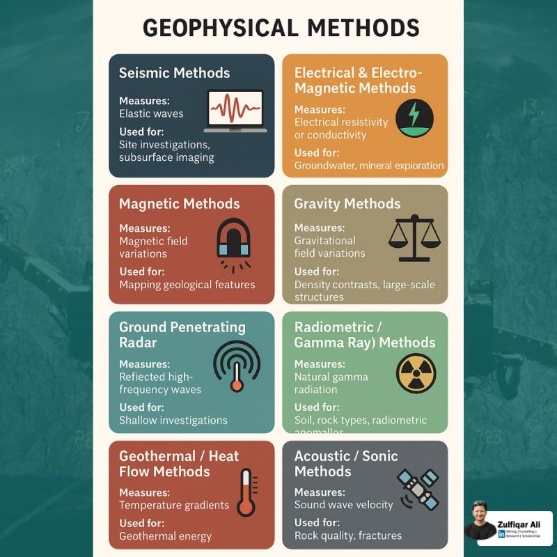
Refraction and MASW are only two of the tools available. The USACE decision matrix (EM 1110-1-1802, Table 2-1) rates each surface method against the question being asked. W = works well in most materials; S = works only under favorable conditions; blank = not recommended.
| Method | Lithology | Top of rock | Rippability | Water table | Faults | Voids / cavities | In-situ moduli | Material boundaries | Buried ferrous objects |
|---|---|---|---|---|---|---|---|---|---|
| Seismic refraction | S | W | W | S | S | W | S | ||
| Seismic reflection | S | S | S | S | S | W | |||
| DC resistivity | S | S | S | S | S | S | S | ||
| Electromagnetics | S | S | S | ||||||
| Ground-penetrating radar | S | S | S | S | S | S | |||
| Gravity | S | S | S | ||||||
| Magnetics | S | W |
Only refraction is rated “works well” for top of rock and rippability; every void-detection method is conditional, which is why karst and mine-void screening on rail corridors normally combines two methods (e.g., resistivity plus microgravity or GPR) and confirms anomalies with borings. USACE also stresses writing explicit objectives into the geophysical contract and including a field-release clause so a method that is not working can be stopped after a short trial near ground truth.
Source: U.S. Army Corps of Engineers (1995). Geophysical Exploration for Engineering and Environmental Investigations. EM 1110-1-1802
| Method | Primary Output | Best Suited Soils | Railroad Application |
|---|---|---|---|
| CPT / CPTu | q_c, f_s, u₂ | Sands to soft clays | Liquefaction screening (UPRR, BNSF); settlement (Amtrak NEC, CSXT) |
| VST | s_u, S_t | Soft to medium clays | Embankment stability (CSXT, CN, G&W); quick clay (CN) |
| PMT | E_PMT, p_L | All soils; rock (SBP) | Foundation modulus (NSR, Amtrak); stiff interbedded soils |
| DMT | I_D, K_D, M_DMT | Soft clays to dense sands | OCR, settlement input (BNSF, CSXT); subgrade assessment |
| MASW | V_s profile, G_max | All soils / rock | Site class, G_max (UPRR, BNSF, CPKC); muskeg thickness (CN) |
| Seismic Refraction | V_P, layer depths | Rock / stiff soils | Depth to rock, rippability (NSR, CPKC, CN) |
Selection hierarchy:
Converting between N and qc is routine when a corridor has old SPT borings and new CPT soundings. A Florida DOT data set (six sites, safety-hammer SPT, electric CPT) shows the limits:
| Soil (USCS) | Linear fit (qc in MPa) | R2 |
|---|---|---|
| Fine sand (SP) | qc = 0.291N + 2.43 | 0.60 |
| Silty fine sand (SM) | qc = 0.12N + 5.0 | 0.35 |
| Silty clayey fine sand (SM/SC) | qc = 0.22N + 2.6 | 0.37 |
| Fine sand with silt (SP-SM) | qc = 0.15N + 7.2 | 0.11 |
| Clayey fine sand (SC) | qc = 0.06N + 5.7 | 0.09 |
Only clean sand gave a usable correlation, and its qc/N ratio matched the published values; sands with more than about 10% fines scattered badly and had higher qc/N than the literature. Treat a converted N or qc as a screening value. For design, calibrate with side-by-side SPT and CPT at a few stations in each geologic unit, and prefer the Robertson soil-behavior-type ratios (above) over a single constant.
Source: Jarushi, F., AlKaabim, S. and Cosentino, P. (2015). “A New Correlation between SPT and CPT for Various Soils.” Int. J. Geological and Environmental Engineering 9(2) · Robertson, P. K. and Cabal, K. L. (2010). Guide to Cone Penetration Testing for Geotechnical Engineering, 4th ed. Gregg Drilling & Testing, Inc.
Only two things need answering. For track subgrade, in situ testing has to establish strength (bearing) and stiffness (deformation), plus where the layering changes. Tests support design in one of two ways:
| Test | Very soft clay | Soft clay | Medium clay | Stiff clay | Silty clay | Silt |
|---|---|---|---|---|---|---|
| Field vane | A | A | B | C | C | D |
| CPT | A | A | A | B | B | C |
| CPTu | A | A | A | B | B | C |
| DMT | A | A | A | A | A | B |
| PMT | B | B | A | A | B | C |
| SPT | D | C | B | A | A | A |
A = high suitability; B = moderate; C = limited; D = not applicable.
Strengths and limitations.
Choosing the test. CPT, vane and DMT depend least on the operator. Where stratigraphy is complex or variable, use more of a cheaper test. Where it is simple, fewer, more expensive tests are acceptable.
After Selig & Waters (1994), chs. 4 and 10. Full reference under Supplemental Sources.
Values from these correlations are estimates, not test results. State the equation ID and source when one is used, confirm the soil or rock is within its range, and calibrate against site testing before design.
Context: We are performing a CPTu sounding to support embankment widening on CSXT's Seaboard Subdivision near Savannah, GA. At a depth of 22 ft, the following data are recorded:
Step 1 — Corrected tip resistance (Eq. 7-1):
q_t = q_c + u₂ × (1 − a)
= 4.20 + 1.80 × (1 − 0.80)
= 4.20 + 0.36
= 4.56 tsf
Step 2 — Total vertical stress:
σ_v = γ × z = 108 pcf × 22 ft = 2,376 psf = 1.188 tsf
Step 3 — Pore water pressure (hydrostatic):
u₀ = γ_w × h_w = 62.4 × (22 − 4) = 62.4 × 18 = 1,123 psf = 0.562 tsf
Step 4 — Effective vertical stress:
σ'_v = σ_v − u₀ = 1.188 − 0.562 = 0.626 tsf
Step 5 — Undrained shear strength (Eq. 7-3, N_kt = 14):
s_u = (q_t − σ_v) / N_kt
= (4.56 − 1.188) / 14
= 3.372 / 14
= 0.241 tsf = 482 psf
Step 6 — Pore pressure ratio (Eq. 7-4):
B_q = (u₂ − u₀) / (q_t − σ_v)
= (1.80 − 0.562) / (4.56 − 1.188)
= 1.238 / 3.372
= 0.367
Interpretation: B_q = 0.37 indicates a normally to lightly overconsolidated soft clay — consistent with Atlantic Coastal Plain alluvium. s_u = 482 psf is consistent with soft to medium clay classification (Chapter 8). This value feeds directly into CSXT embankment stability analysis (Chapter 13, Bishop Simplified method).
Values from these correlations are estimates, not test results. State the equation ID and source when one is used, confirm the soil or rock is within its range, and calibrate against site testing before design.
Context: CN requires VST data to assess embankment stability adjacent to a soft lacustrine clay deposit near the south shore of Lake Erie. VST results at 18 ft depth:
Step 1 — Peak s_u (Eq. 7-6):
s_u (peak) = 6 × T_peak / (7 × π × D³)
= 6 × 12.4 / (7 × 3.1416 × 0.187³)
= 74.4 / (7 × 3.1416 × 0.00654)
= 74.4 / 0.14397
= 516.8 psf = 0.258 tsf
Step 2 — Remolded s_u:
s_u (remolded) = 6 × 3.1 / (7 × π × 0.187³)
= 18.6 / 0.14397
= 129.2 psf
Step 3 — Sensitivity (Eq. 7-8):
S_t = 516.8 / 129.2 = 4.0
S_t = 4.0 — medium sensitivity. CN's trigger for enhanced seismic review is S_t > 8; this site does not trigger that requirement.
Step 4 — Bjerrum correction (Eq. 7-7, PI = 55%, μ = 0.78 interpolated):
s_u (design) = 0.78 × 0.258 = 0.201 tsf = 402 psf
Interpretation: Design s_u = 402 psf is used in the slope stability model (Chapter 13). Uncorrected vane data (516 psf) would have overestimated embankment stability by approximately 29%. Per CN Engineering Standards, Bjerrum correction is mandatory for all VST data used in embankment design.
Context: UPRR requires AASHTO seismic site classification for a new intermodal facility in the Mid-Continent region. MASW inversion yields:
| Layer | Thickness d_i (ft) | V_si (ft/s) |
|---|---|---|
| 1 | 12 | 480 |
| 2 | 28 | 920 |
| 3 | 35 | 1,650 |
| 4 | 25 | 3,200 |
Total depth = 100 ft. Apply Equation 7-16:
Numerator: Σd_i = 12 + 28 + 35 + 25 = 100 ft
Denominator: Σ(d_i / V_si):
= 12/480 + 28/920 + 35/1,650 + 25/3,200
= 0.02500 + 0.03043 + 0.02121 + 0.00781
= 0.08445 s/ft × ft = 0.08445 s
V_s,30 = 100 / 0.08445 = 1,185 ft/s
Site Class D (600–1,200 ft/s — stiff soil). Per AREMA MRE Chapter 8 and UPRR Engineering Instruction Manual, Site Class D triggers the use of site amplification factors F_a and F_v in seismic design. G_max for the upper layer:
G_max = (120/32.2) × 480² = 3.727 × 230,400 = 858,893 psf ≈ 429 tsf
This is the baseline stiffness for subgrade support under 286K–315K GRL loading.
| Depth (ft) | q_c (tsf) | f_s (psi) | u₂ (psi) | R_f (%) | SBT Zone | s_u (psf) | B_q |
|---|---|---|---|---|---|---|---|
| 5 | 3.1 | 0.30 | 8.2 | 1.04 | 4 — Silt mix | 382 | 0.28 |
| 10 | 2.4 | 0.48 | 11.6 | 2.31 | 3 — Clay | 298 | 0.42 |
| 15 | 1.8 | 0.54 | 14.3 | 3.46 | 3 — Clay | 224 | 0.59 |
| 20 | 1.6 | 0.61 | 16.1 | 4.17 | 1 — Sensitive clay | 199 | 0.72 |
| 25 | 2.1 | 0.44 | 13.8 | 2.41 | 3 — Clay | 262 | 0.48 |
| 30 | 8.7 | 0.32 | 9.4 | 0.42 | 6 — Clean sand | — | 0.04 |
| 35 | 22.4 | 0.18 | 7.6 | 0.09 | 8 — Dense sand | — | 0.01 |
B_q > 0.5 at 15–20 ft depth indicates soft, sensitive clay layer — triggers VST verification per BNSF Engineering Instructions for soft-ground embankment design.
Reference graphics
Values from these correlations are estimates, not test results. State the equation ID and source when one is used, confirm the soil or rock is within its range, and calibrate against site testing before design.
Checklist · Part V · Subsurface Exploration
Pre-Mobilization
During Testing
Post-Testing
Values from these correlations are estimates, not test results. State the equation ID and source when one is used, confirm the soil or rock is within its range, and calibrate against site testing before design.
Question 3-1 A CPTu sounding on an NSR bridge approach fill yields the following at 30 ft depth: q_c = 6.80 tsf, u₂ = 0.95 tsf, net area ratio a = 0.82, total stress σ_v = 1.95 tsf. Calculate (a) corrected tip resistance q_t and (b) undrained shear strength s_u using N_kt = 13.
Answer 3-1: (a) q_t = q_c + u₂ × (1 − a) = 6.80 + 0.95 × (1 − 0.82) = 6.80 + 0.171 = 6.971 tsf (b) s_u = (q_t − σ_v) / N_kt = (6.971 − 1.95) / 13 = 5.021 / 13 = 0.386 tsf = 772 psf This s_u would be classified as medium clay (Chapter 8) and is suitable input for NSR bridge abutment bearing capacity calculations (Chapter 11).
Question 3-2 A VST at 12 ft depth in a CN lacustrine clay deposit yields T_peak = 8.6 lb·ft and T_remolded = 1.4 lb·ft. Standard vane D = 0.187 ft. Plasticity Index = 70%. Calculate (a) peak s_u, (b) sensitivity S_t, (c) design s_u after Bjerrum correction, and (d) determine whether CN's enhanced seismic review is triggered.
Answer 3-2: (a) s_u (peak) = 6 × 8.6 / (7 × π × 0.187³) = 51.6 / 0.14397 = 358.4 psf = 0.179 tsf (b) s_u (remolded) = 6 × 1.4 / 0.14397 = 58.3 psf; S_t = 358.4 / 58.3 = 6.1 (c) μ for PI = 70%: interpolate between 65% (μ = 0.72) and 80% (μ = 0.65) → μ ≈ 0.70; s_u (design) = 0.70 × 0.179 = 0.125 tsf = 250 psf (d) S_t = 6.1 < 8.0 — CN's enhanced seismic review threshold is not triggered, but the site is classified as sensitive and warrants careful embankment load staging.
Question 3-3 An MASW survey on a BNSF soft-ground site yields V_s,30 = 580 ft/s. The upper soil layer has γ = 110 pcf and V_s = 410 ft/s. Determine (a) AASHTO site class, (b) G_max for the upper layer in tsf, and (c) the significance for BNSF Engineering Instructions.
Answer 3-3: (a) V_s,30 = 580 ft/s < 600 ft/s → Site Class E (soft clay) (b) ρ = 110 / 32.2 = 3.416 slug/ft³; G_max = 3.416 × 410² = 3.416 × 168,100 = 574,390 psf / 2,000 = 287 tsf (c) Site Class E requires BNSF to apply maximum seismic amplification factors (F_a and F_v) per AREMA MRE Chapter 8, and BNSF Engineering Instructions require a site-specific seismic response analysis rather than the standard code-based approach. Additionally, G_max = 287 tsf indicates a very soft subgrade; BNSF's track modulus specifications for this corridor may require ground improvement (Chapter 17) before track installation.
Question 3-4 Seismic refraction on an NSR rock cut project yields V₁ = 3,800 ft/s, V₂ = 9,200 ft/s, and crossover distance x_c = 48 ft. Calculate (a) depth to rock and (b) whether blasting is required per the rippability table.
Answer 3-4: (a) Using Equation 7-18:
h = (48/2) × √((9,200 − 3,800)/(9,200 + 3,800))
= 24 × √(5,400 / 13,000)
= 24 × √0.4154
= 24 × 0.6445
= 15.5 ft
Depth to rock ≈ 15.5 ft. (b) V₂ = 9,200 ft/s falls in the "Difficult" rippability category (8,000–12,000 ft/s); blasting is likely required. NSR's Engineering Standards Manual requires advance notification to NSR ROW management and coordination with state explosive use permits before blasting within 200 ft of active track.
Question 3-5 A DMT at 14 ft depth in a CSXT embankment foundation yields corrected pressures p_0 = 1,240 psf and p_1 = 3,860 psf. Effective vertical stress σ'_v = 780 psf; hydrostatic u₀ = 0. Calculate (a) I_D, (b) K_D, (c) E_D, and (d) M_DMT. Classify the soil type.
Answer 3-5: (a) I_D = (p_1 − p_0) / (p_0 − u₀) = (3,860 − 1,240) / (1,240 − 0) = 2,620 / 1,240 = 2.11 → Sand (I_D > 1.8) (b) K_D = (p_0 − u₀) / σ'_v = 1,240 / 780 = 1.59 (c) E_D = 34.7 × (p_1 − p_0) = 34.7 × 2,620 = 90,914 psf ≈ 45.5 tsf (d) For sand (I_D > 3.0): R_M = 1.0; M_DMT = 1.0 × 90,914 = 90,914 psf ≈ 45.5 tsf K_D = 1.59 ≈ K₀ for NC sand; OCR ≈ (1.59/1.5)^1.56 ≈ 1.09 — essentially normally consolidated. This M_DMT value is input to the immediate settlement calculation for the CSXT embankment widening (Chapter 12).
Values from these correlations are estimates, not test results. State the equation ID and source when one is used, confirm the soil or rock is within its range, and calibrate against site testing before design.
Authors: Daniel P. Colwell and Mario Ruel. This chapter was written and compiled by Daniel P. Colwell and Mario Ruel for Railway Ground Hazard Risk Management.
Technical content is drawn from the published sources below, and credit for that material belongs to their authors and publishers. Tables, equations and figures taken from a specific source are also cited where they appear.
File locations for these documents are listed under Supplemental Sources — LEVI Library.
Material in the green “Supplemental reference” boxes throughout this chapter was added from the following documents in the LEVI geotechnical library. Text is summarized or paraphrased; tables are reproduced with their original source noted; figures are reproduced from the cited document for internal reference use. Consult the original document before relying on a value for design. Blocks marked “After Selig & Waters (1994)” summarize item S7 for railroad clients; tables are condensed from the book and its figures are not reproduced.